Beta Distribution Calculator

This beta distribution calculator can help you discover one of the most useful families of probability distributions; namely, the beta family! This tool can produce various beta distribution graphs, including the plots of both probability density and cumulative distribution functions (pdf and cdf) of beta distribution, as well as compute probabilities and common measures, such as the mean and variance of beta distributions.

If you are only now discovering what beta distribution is all about, scroll down to find a short (yet comprehensive) article, which also provides you with a complete set of formulas for beta distribution, in case you ever need to perform some calculations by hand.

What is beta distribution?

Beta distribution is, in fact, a whole family of continuous distributions on the interval [0, 1] . What is important is that the shapes of distributions belonging to this family vary widely. They can be symmetric, skewed, unimodal, bimodal, etc. Somewhat surprisingly, all this variety is encoded in just two real positive numbers, α and β , which control the shape, and so they are called shape parameters.

As a consequence, beta distribution is very common in a variety of applications because it is so flexible. In this article, you'll see several examples of beta distribution shapes. To better understand how it all works mathematically, we'll now move on to the beta distribution formulas.

The pdf of beta distribution

The probability density function (pdf) of beta distribution is given by the following formula:

f ( x ) = const ⋅ x α − 1 ⋅ ( 1 − x ) β − 1 \small f(x) = \textrm\cdot x^ \cdot (1-x)^ f ( x ) = const ⋅ x α − 1 ⋅ ( 1 − x ) β − 1

where const is a constant depending on α and β that provides normalization, i.e., ensures that the total probability (the area under the pdf) is equal to 1 . This constant can be expressed by the gamma function, Γ as:

or via the beta function, B as:

Both beta and gamma functions are special functions defined with integrals. Check out our gamma function calculator to discover more if you wish. However, you don't need to worry much about the value of the normalizing constant: what really matters is the shape of the distribution, and the shape is encoded in the other part of the pdf formula, i.e., in x α − 1 ⋅ ( 1 − x ) β − 1 x^ \cdot (1-x)^ x α − 1 ⋅ ( 1 − x ) β − 1 .

In contrast to the pdf, the cdf of the beta distribution (also called the incomplete beta function) as well as its quantile function (the inverse of cdf) cannot be expressed by simple formulas.

How to use this beta distribution calculator?

Formulas for beta distribution can be complicated, but don't worry! Our beta distribution calculator can help you at any time. Here's a quick instruction on how to use this tool:

1. Choose the mode of the calculator. There are six options available:
   • Probability calculator;
   • Sample generator;
   • Probability distribution function (pdf of beta distribution);
   • Cumulative density function (cdf of beta distribution);
   • Quantile function; or
   • Common measures.
2. For the Probability calculator mode, you must also select a probability type.
3. Enter the shape parameters α and β of the beta distribution you want to consider.
4. In the case of probability, cdf, pdf, and quantile, enter the value of the argument. It must be a number between 0 and 1 .
5. In the case of the sample generator, choose how many numbers are to be generated.
6. Enjoy the results returned by Omni's beta distribution calculator 🙂!

If you play a bit with our beta distribution calculator, you will notice that this family of probability distributions does indeed have a lot of different pdf shapes. In what follows, we will show you a bunch of beta distribution graphs. How many of them have you managed to find on your own?

Examples of beta distribution graphs

As we've mentioned, the pdf of beta distribution looks different for different values of the shape parameters α , β . Possible shapes include:

• Straight lines;
• U-shapes;
• Bell-shapes (similar to normal distribution); and
• J-shapes.

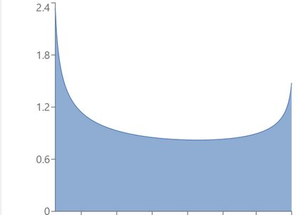
We'll talk first about symmetric and then about and skewed beta distributions. It's useful to remember that:

• If α = β , then the density function is symmetric (and the symmetry axis is x = ½ ).
• If α ≠ β , then the density function is skewed.

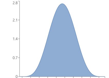
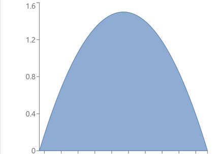
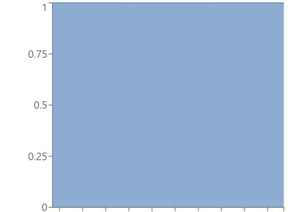
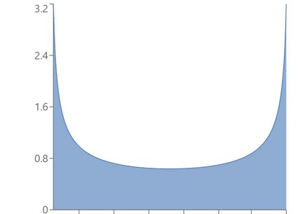
Here are several examples of symmetric beta distribution plots:

• α = β = 6 : Bell-shaped distribution

• α = β = 2 : Parabolic distribution

• α = β = 1 : Standard uniform distribution

• α = β = 0.5 : U-shaped distribution

• In the limit α = β → 0 we arrive at the Bernoulli distribution with equal probability 1/2 for x = 0 and x = 1 . That is, we get the coin flip! See our coin flip probability calculator to learn more.
• In the limit α = β → ∞ we arrive at the Dirac delta at 1/2 , i.e., the probability of getting 1/2 is 1 (this outcome is certain), and the probability of any other outcome is 0 (any other outcome is impossible).

And here are some examples of skewed (non-symmetric) beta distribution plots.

• α = 0.7, β = 0.8 : Skewed U-shaped distribution

• α = 2, β = 5 : Unimodal distribution

• α = 0.5, β = 2 : J-shaped distribution

• α = 1, β = 2 : Inclined straight line distribution

• α = 1, β = 5 : Strictly decreasing distribution

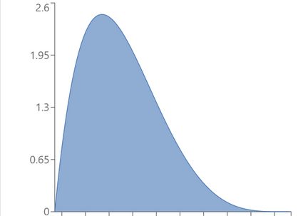
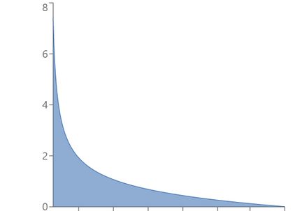
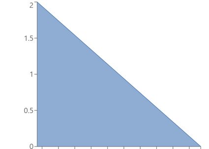
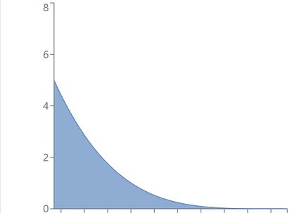
If we swap the parameters, we will obtain the mirror image of the initial pdf (more formally, the image of symmetry about the axis x = 1/2 ) - use the beta distribution calculator to verify this claim! Also, note that all the skewed distributions above are right-tailed, i.e., they have positive skewness because the parameters satisfy a < b (see also the skewness formula). Their mirror images would be left-tailed.

Clearly, for different values of α and β , it is not only the shape of pdf that changes but also the values of distribution measures. In the next section, you can find the formulas for the mean and variance of beta distribution and for some other common measures.

Mean of beta distribution (and other measures)

In this section, you can find the formulas for various measures of beta distribution, depending on the values of the shape parameters α and β .

• Mean of beta distribution:

• In general, the median of beta distribution cannot be expressed with a simple formula. For the symmetric case (i.e., when α = β ), the median is of course equal to 0.5 .
• If α, β > 1 , then the mode of beta distribution has the following formula:

• Variance of beta distribution:

• Skewness of beta distribution:

2 ( β − α ) α + β + 1 ( α + β + 2 ) α β \footnotesize \qquad \frac><(\alpha + \beta+2)\sqrt<\alpha\beta>> ( α + β + 2 ) α β

​ 2 ( β − α ) α + β + 1

🙋 See the skewness calculator if you haven't encountered this notion yet!

Why is beta distribution popular in Bayesian inference?

Beta distribution is very often chosen as the prior distribution because it is a conjugate prior for a bunch of likelihoods. That is, the posterior distribution will also be a beta distribution and, having carried out the experiment, we only need to update the parameters α and β by adding the number of successes and failures to the initial parameters, respectively.

Beta distribution is the conjugate prior for the following distributions:

• Binomial;
• Negative binomial; and
• Geometric.

Exploiting this feature of beta distribution allows us to avoid computing the posterior directly from the Bayesian formula, which can be numerically expensive.

FAQ

How do I calculate the expected value in a beta distribution?

To determine the expected value of a random variable X following the beta distribution with shape parameters α and β , use the formula:

How do I check if a beta distribution is symmetric?

The skewness of beta distribution depends on the two shape parameters α and β :

• If α = β , then beta distribution is symmetric (has zero skewness).
• If α < β then beta distribution is right-skewed (positive skewness).
• If α > β then beta distribution is left-skewed (negative skewness).